G..1 Python

(しばらく工事中)

とりあえず、以前書いたメモ「Pythonでode」にリンクを張っておく。

scipy のodeint() は、定評のある ODEPACK を利用しているそうである。

「scipy.integrate.odeint」

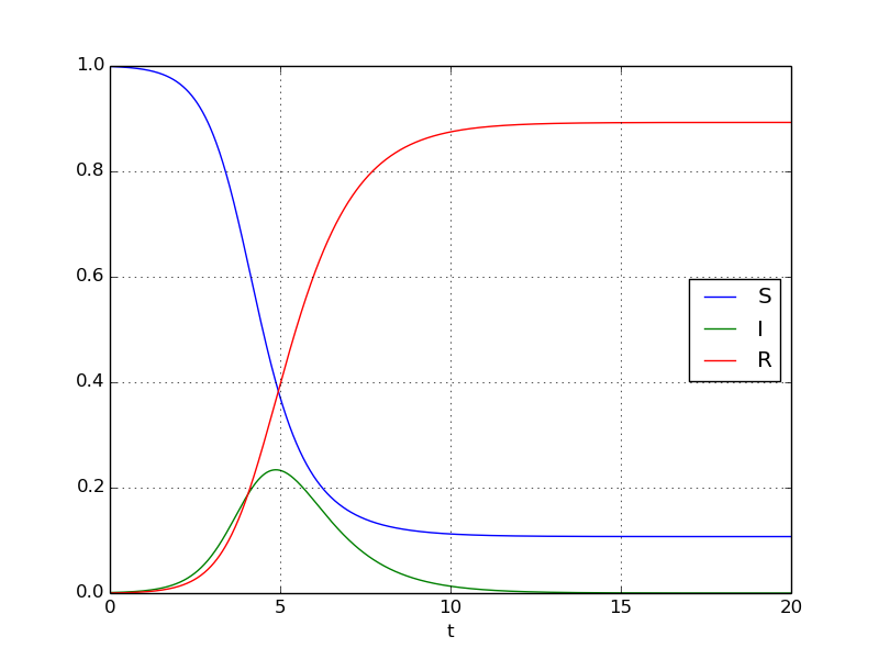
testsir2.py

# testsir2.py # import numpy as np from scipy.integrate import odeint import matplotlib.pyplot as plt # x=(S,I,R) def sir(x, t, R0): return [-R0*x[0]*x[1], R0*x[0]*x[1]-x[1], x[1]] R0=2.5 I0=0.001 x0=[1.0-I0,I0,0.0] n=1000 t=np.linspace(0.0, 20.0, n+1) x=odeint(sir, x0, t, args=(R0,)) plt.plot(t,x[:,0],'b', label='S') plt.plot(t,x[:,1],'g', label='I') plt.plot(t,x[:,2],'r', label='R') plt.legend(loc='best') plt.xlabel('t') plt.grid() plt.show()

**図 18:** 無次元化SIRモデルの解曲線 (, )

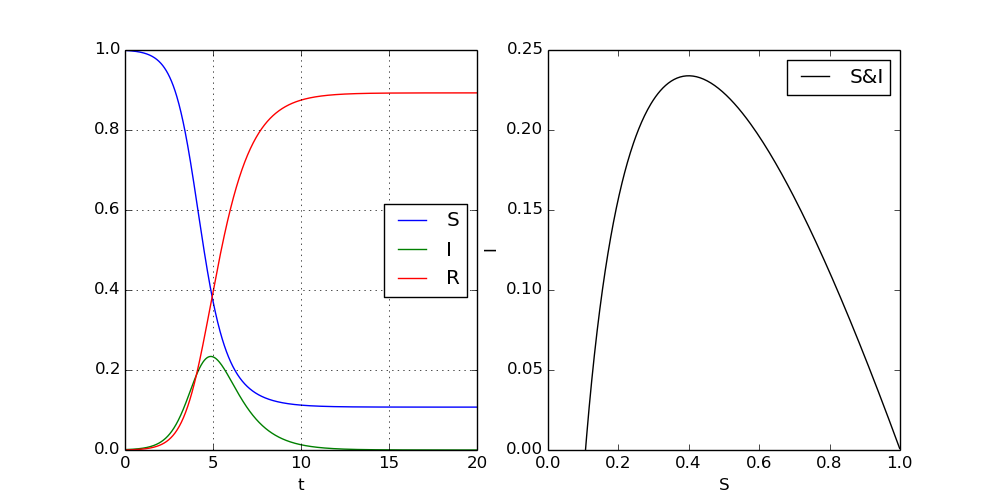
簡単に書けるのは嬉しい。ついでにSI平面上で解の軌道を描いてみる。

testsir3.py

# testsir3.py --- SIR model # coding: utf-8 # import numpy as np from scipy.integrate import odeint import matplotlib.pyplot as plt # x=(S,I,R) def sir(x, t, R0): return [-R0*x[0]*x[1], R0*x[0]*x[1]-x[1], x[1]] R0=2.5 I0=0.001 x0=[1.0-I0,I0,0.0] n=1000 t=np.linspace(0.0, 20.0, n+1) x=odeint(sir, x0, t, args=(R0,)) plt.figure(figsize=(10,5)) plt.subplot(121) plt.plot(t,x[:,0],'b', label='S') plt.plot(t,x[:,1],'g', label='I') plt.plot(t,x[:,2],'r', label='R') plt.legend(loc='best') plt.xlabel('t') plt.grid() plt.subplot(122) plt.xlim(0.0,1.0) plt.plot(x[:,0],x[:,1],'k',label='S&I') plt.legend(loc='best') plt.xlabel('S') plt.ylabel('I') plt.show()

**図 19:** 無次元化SIRモデルの解曲線と解軌道 (, )

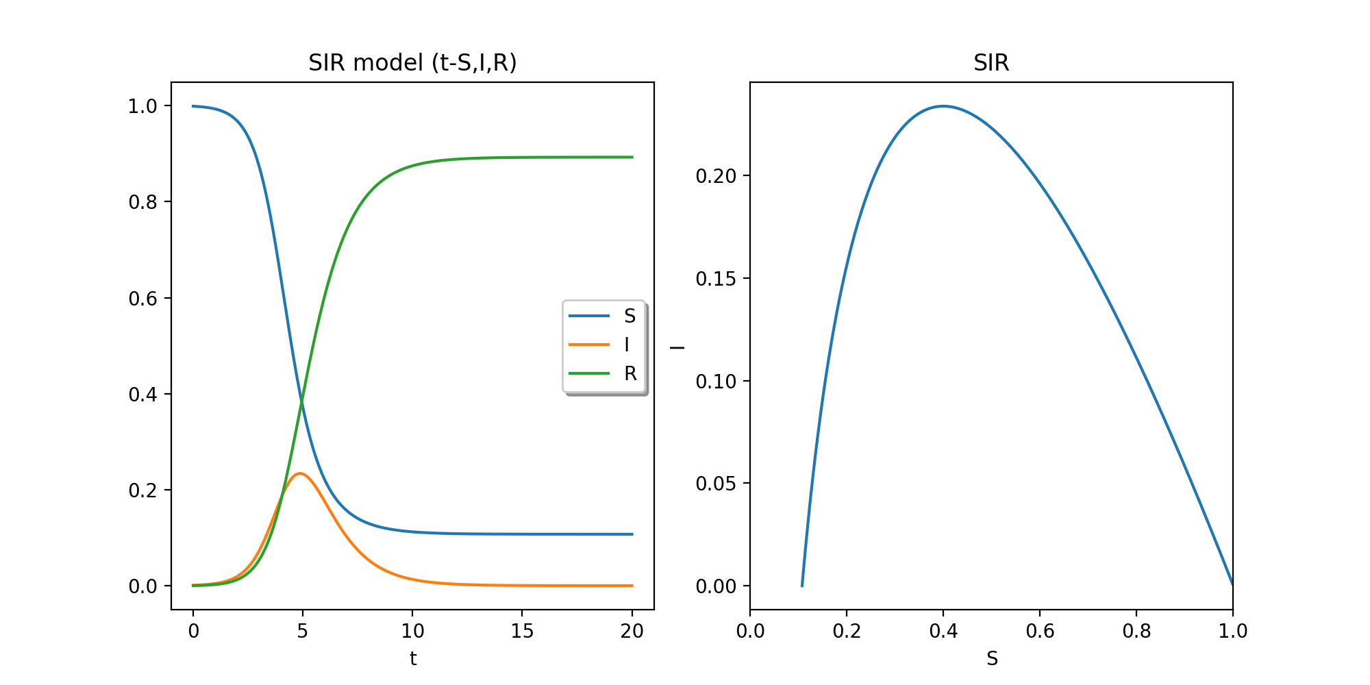
新しく用意した、という scipy.integrate.solve_ivp を利用するプログラムは、以下のようになる。

testsir4.py

# testsir4.py --- SIR model # coding: utf-8 # import numpy as np from scipy.integrate import solve_ivp import matplotlib.pyplot as plt # x=(S,I,R) def sir(t, x, R0): return [-R0*x[0]*x[1], R0*x[0]*x[1]-x[1], x[1]] R0=2.5 I0=0.001 x0=[1.0-I0,I0,0.0] T=20.0 sol=solve_ivp(sir, [0.0, T], x0, args=(R0,), dense_output=True, rtol=1e-10,atol=1e-10) n=1000 t=np.linspace(0.0, T, n+1) x = sol.sol(t) plt.figure(figsize=(10,5)) plt.subplot(121) plt.plot(t,x.T) plt.xlabel('t') plt.legend(['S', 'I', 'R'], shadow=True) plt.title('SIR model (t-S,I,R)') plt.subplot(122) plt.xlim(0.0,1.0) plt.plot(x[0], x[1], "-") plt.xlabel("S") plt.ylabel("I") plt.title("SIR") plt.show()

**図 20:** 無次元化SIRモデルの解曲線と解軌道 (, )

sir() の引数の順番は odeint() のときとは変える必要がある。 dense_output=True, rtol=1e-10,atol=1e-10 のあたりは、実は見様見真似で、どうするべきか、まだよく理解していない。

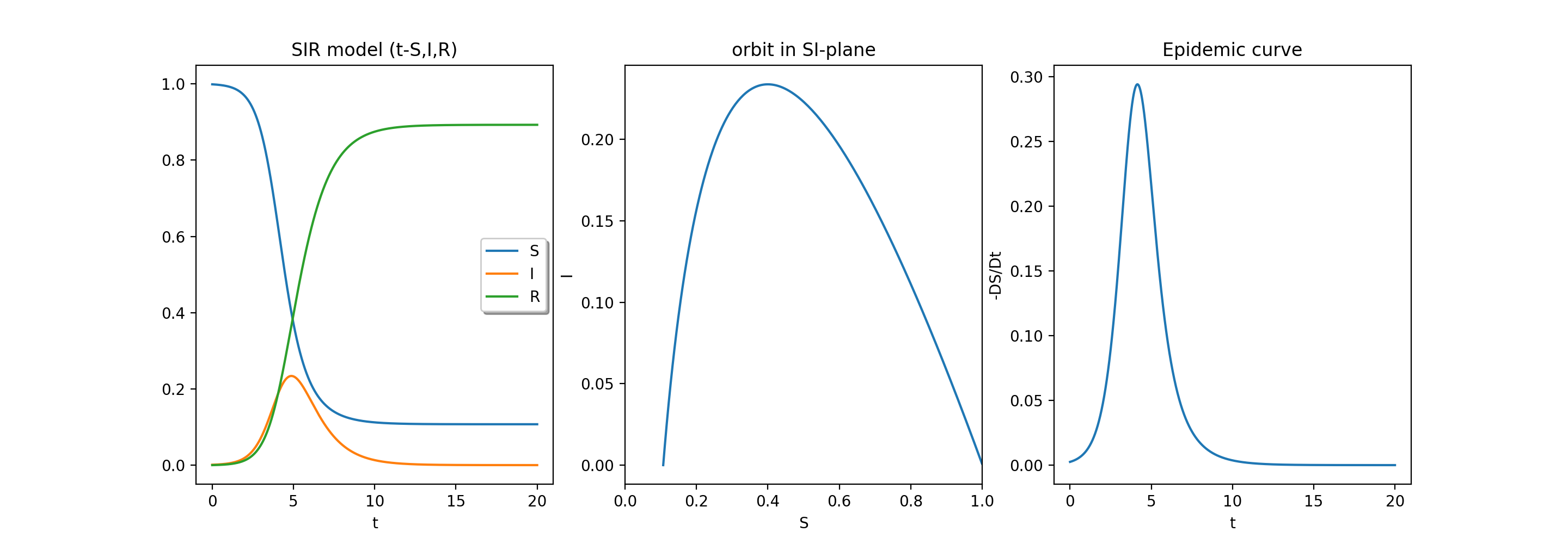
そうだ、流行曲線というのも描いてみよう。これは新規感染者数の時間経過を表すものである。 $-\frac{\D S}{\D t}$ , つまりを描けば良い。

testsir5.py

# testsir5.py --- SIR model # coding: utf-8 # import numpy as np from scipy.integrate import solve_ivp import matplotlib.pyplot as plt # x=(S,I,R) def sir(t, x, R0): return [-R0*x[0]*x[1], R0*x[0]*x[1]-x[1], x[1]] R0=2.5 I0=0.001 x0=[1.0-I0,I0,0.0] T=20.0 sol=solve_ivp(sir, [0.0, T], x0, args=(R0,), dense_output=True, rtol=1e-10,atol=1e-10) n=1000 t=np.linspace(0.0, T, n+1) x = sol.sol(t) plt.figure(figsize=(15,5)) plt.subplot(131) plt.plot(t,x.T) plt.xlabel('t') plt.legend(['S', 'I', 'R'], shadow=True) plt.title('SIR model (t-S,I,R)') plt.subplot(132) plt.xlim(0.0,1.0) plt.plot(x[0], x[1], "-") plt.xlabel("S") plt.ylabel("I") plt.title("orbit in SI-plane") plt.subplot(133) plt.plot(t,R0*x[0]*x[1],"-") plt.xlabel('t') plt.ylabel('-DS/Dt') plt.title("Epidemic curve") plt.show()

**図 21:** 無次元化SIRモデルの解曲線, 解軌道, 流行曲線 (, )

古い Python 環境しかインストールしていなくて、 solve_ivp() が使えない人が、結構大勢いることに気づいた (何か勧めるときは、アップデートの仕方を教えてあげるべきだ)。ともあれ、odeint() で上と同じことをするには、次のようなプログラムを使えば良い。
testsir5b.py

# testsir5b.py --- SIR model # coding: utf-8 # import numpy as np from scipy.integrate import odeint import matplotlib.pyplot as plt # x=(S,I,R) def sir(x, t, R0): return [-R0*x[0]*x[1], R0*x[0]*x[1]-x[1], x[1]] R0=2.5 I0=0.001 x0=[1.0-I0,I0,0.0] n=1000 t=np.linspace(0.0, 20.0, n+1) x=odeint(sir, x0, t, args=(R0,)) plt.figure(figsize=(15,5)) plt.subplot(131) plt.plot(t,x[:,0],'b', label='S') plt.plot(t,x[:,1],'g', label='I') plt.plot(t,x[:,2],'r', label='R') plt.legend(loc='best') plt.xlabel('t') plt.title('SIR model (t-S,I,R)') plt.grid() plt.subplot(132) plt.xlim(0.0,1.0) plt.plot(x[:,0],x[:,1],'k',label='S&I') plt.legend(loc='best') plt.xlabel('S') plt.ylabel('I') plt.title("orbit in SI-plane") plt.subplot(133) plt.plot(t,R0*x[:,0]*x[:,1],'b', label='S') plt.xlabel('t') plt.ylabel('-DS/Dt') plt.title("Epidemic curve") plt.show()

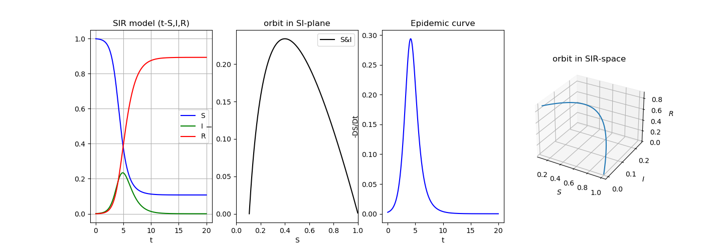
ついでに3次元相空間での軌道も描いてみる。

testsir6.py

# testsir6.py --- SIR model # coding: utf-8 # import numpy as np from scipy.integrate import odeint import matplotlib.pyplot as plt # x=(S,I,R) def sir(x, t, R0): return [-R0*x[0]*x[1], R0*x[0]*x[1]-x[1], x[1]] # R0=2.5 I0=0.001 x0=[1.0-I0,I0,0.0] n=1000 t=np.linspace(0.0, 20.0, n+1) x=odeint(sir, x0, t, args=(R0,)) fig=plt.figure(figsize=(20,5)) # S,I,Rの時間変化 plt.subplot(141) plt.plot(t,x[:,0],'b', label='S') plt.plot(t,x[:,1],'g', label='I') plt.plot(t,x[:,2],'r', label='R') plt.legend(loc='best') plt.xlabel('t') plt.title('SIR model (t-S,I,R)') plt.grid() # SI平面での軌道 plt.subplot(142) plt.xlim(0.0,1.0) plt.plot(x[:,0],x[:,1],'k',label='S&I') plt.legend(loc='best') plt.xlabel('S') plt.ylabel('I') plt.title("orbit in SI-plane") # 流行曲線 plt.subplot(143) plt.plot(t,R0*x[:,0]*x[:,1],'b', label='S') plt.xlabel('t') plt.ylabel('-DS/Dt') plt.title("Epidemic curve") # SIR空間での軌道 # 3DAxesを追加 ax = fig.add_subplot(144, projection='3d') # 軸ラベルを設定 ax.set_xlabel("$S$") ax.set_ylabel("$I$") ax.set_zlabel("$R$") #曲線を描画 ax.plot(x[:, 0], x[:, 1], x[:, 2]) plt.title("orbit in SIR-space") plt.show()

**図 22:** 無次元化SIRモデルと4つの可視化

桂田祐史