26 Pythonでode

(しばらく工事中。あまり Mac と関係ないかな。)

結局は scipy を使うことになるのかな。まずは scipy.integrate.odeint なのだろうか。

「Integration and ODEs (scipy.integrate)¶」

(そういえば数値積分もあるわけか。クラシックなものの名前が見えるけれど、 DE はないのかな？○先生とか誰か書かないかな。)

Solving initial value problems for ODE systems には、

The solvers are implemented as individual classes, which can be used directly (low-level usage) or through a convenience function.

と書いてあって、以下のものがあげられている。

solve_ivp(fun, t_span, y0[, method, t_eval, ])
scipy.integrate.solve_ivp
ここは一度時間をかけて読むべきか。使い方を調べないと。
RK23(fun, t0, y0, t_bound[, max_step, rtol, …])
RK45(fun, t0, y0, t_bound[, max_step, rtol, …])
DOP853(fun, t0, y0, t_bound[, max_step, …])
Radau(fun, t0, y0, t_bound[, max_step, …])
BDF(fun, t0, y0, t_bound[, max_step, rtol, …])
LSODA(fun, t0, y0, t_bound[, first_step, …])

つい古い方から調べたくなる。 Old API については

These are the routines developed earlier for SciPy. They wrap older solvers implemented in Fortran (mostly ODEPACK). While the interface to them is not particularly convenient and certain features are missing compared to the new API, the solvers themselves are of good quality and work fast as compiled Fortran code. In some cases, it might be worth using this old API.

これらは以前にSciPy用に開発されたルーチンです。これらはFortranで実装された古いソルバー（主にODEPACK）をラップしています。新しいAPIに比べて、インターフェースは特に便利ではなく、いくつかの機能が欠けていますが、ソルバー自体は質が高く、 Fortranのコンパイル済みコードとして高速に動作します。場合によっては，この古いAPIを使う価値があるかもしれません．

odeint(func, y0, t[, args, Dfun, col_deriv, …]) -- Integrate a system of ordinary differential equations.
ode(f[, jac]) -- A generic interface class to numeric integrators.
complex_ode(f[, jac]) -- A wrapper of ode for complex systems.

と書いてある。謙虚ですね。なるほど ODEPACK ですか。参考文献表もきちんとしているし (PDFへのリンク付きだ)、学ぶべきものかも。

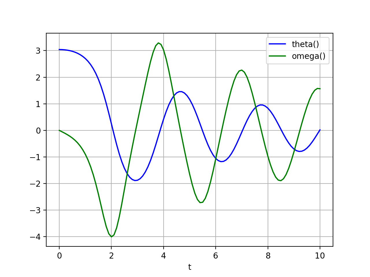
scipy.integrate.odeint にある例を。

(1)	$\displaystyle \theta''(t)+b\theta'(t)+c*\sin\theta(t)=0.$

(速度に比例する抵抗を受ける単振子？) 一階の微分方程式に直す。

(2)		$\displaystyle \theta'(t)=\omega(t),$
(3)		$\displaystyle \omega'(t)=-b\omega(t)-c\sin\theta(t).$

# testodeint.py
# https://docs.scipy.org/doc/scipy/reference/generated/scipy.integrate.odeint.html
import numpy as np
from scipy.integrate import odeint
import matplotlib.pyplot as plt

def pend(y, t, b, c):
    theta, omega = y
    dydt = [omega, -b*omega - c*np.sin(theta)]
    return dydt

b=0.25
c=5.0

y0=[np.pi-0.1,0.0]
t=np.linspace(0,10,101)

sol=odeint(pend, y0, t, args=(b,c))

plt.plot(t,sol[:,0],'b', label='theta()')
plt.plot(t,sol[:,1],'g', label='omega()')
plt.legend(loc='best')
plt.xlabel('t')
plt.grid()
plot.show()

なるほど pend() とするのは、やはりpendulum だからだろう。 $\pi-0.1$ というのはずいぶん威勢が良いですね (ほぼ真上、あまりリアリスティックでない)。 np.linspace() で (100 でなくて) 101 となっているのを見るのは、ほっとする。 sol は2次元配列で、

という shape であると (1次元配列だと要素数という言葉があるけれど、多次元配列では何と言うのかな。)。 args=(b,c) というようなことが出来るのは知らなかった。デフォールトは4次の Runge-Kutta 法みたい。

図: 空気抵抗を受ける振り子の運動 (角度と角速度), `https://docs.scipy.org/doc/scipy/reference/generated/scipy.integrate.odeint.html`

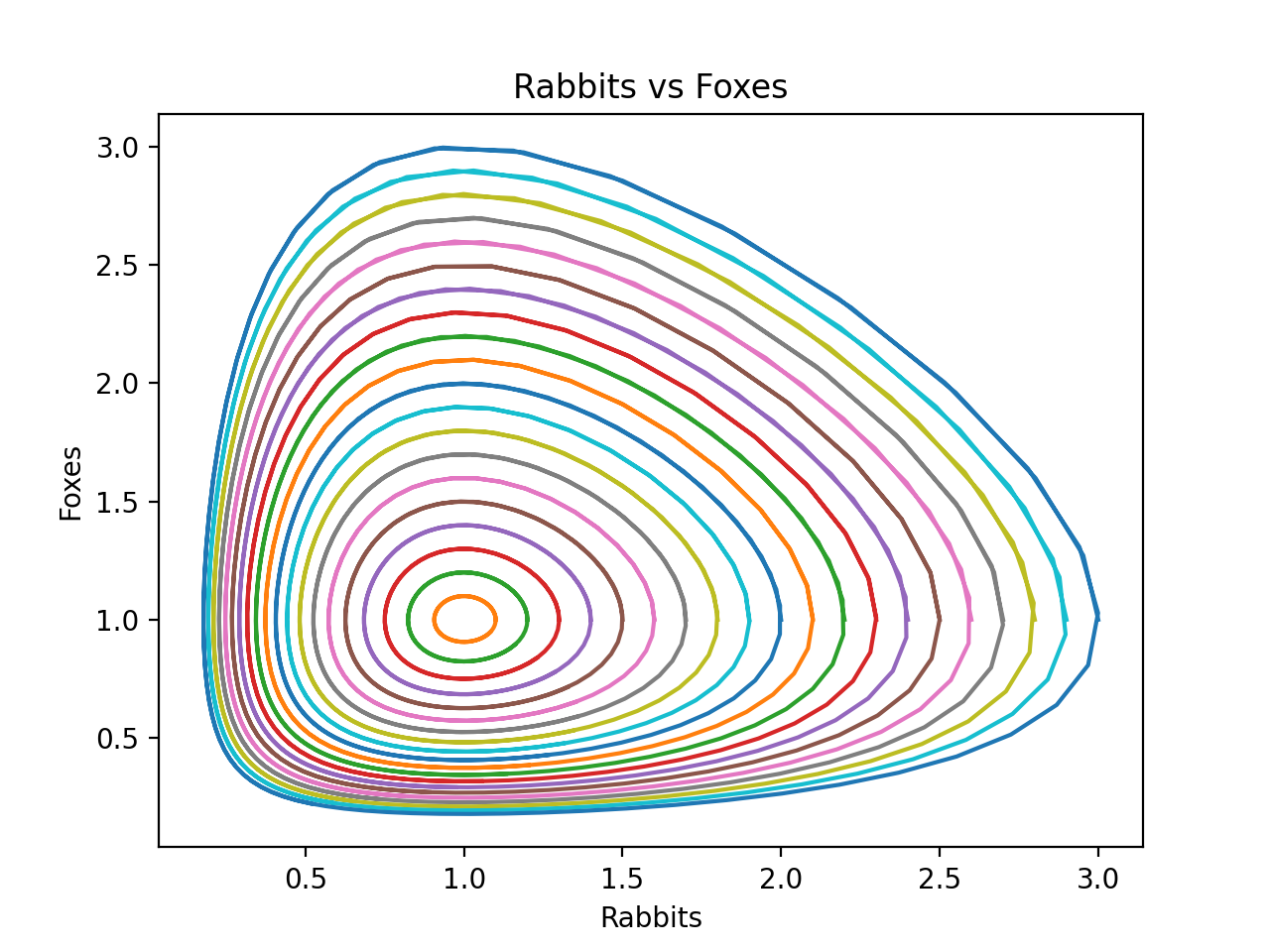
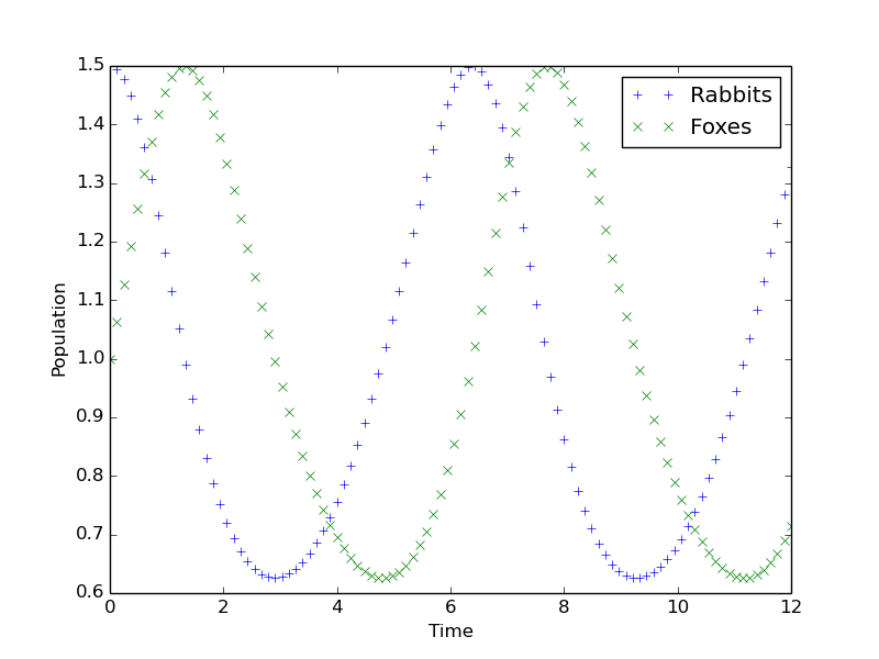
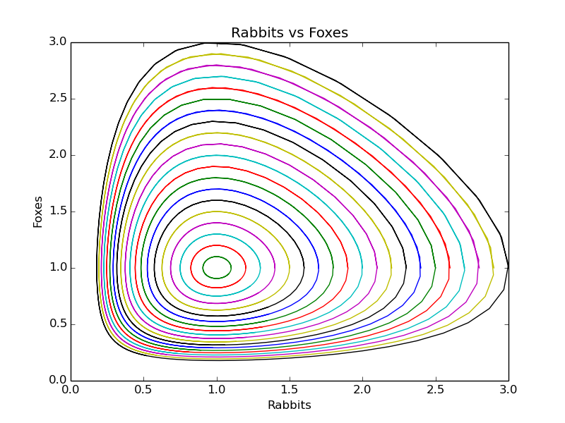
Example: Solving Ordinary Differential Equations にある例を。うさぎと狐とあるけれど、これは Lotka-Volterra 方程式だ。

# testodeint2.py # coding: utf_8 # https://sam-dolan.staff.shef.ac.uk/mas212/notebooks/ODE_Example.html # # Import the required modules import numpy as np import matplotlib.pyplot as plt # This makes the plots appear inside the notebook #%matplotlib inline from scipy.integrate import odeint a,b,c,d = 1,1,1,1 def dP_dt(P, t): return [P[0]*(a - b*P[1]), -P[1]*(c - d*P[0])] ts = np.linspace(0, 12, 100) # 0<=t<=8 で閉じる。100点は粗いかも。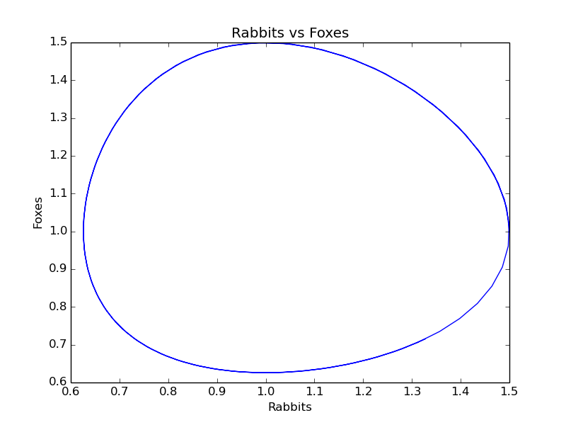 P0 = [1.5, 1.0] Ps = odeint(dP_dt, P0, ts) prey = Ps[:,0] predators = Ps[:,1] plt.plot(ts, prey, "+", label="Rabbits") plt.plot(ts, predators, "x", label="Foxes") plt.xlabel("Time") plt.ylabel("Population") plt.legend() plt.show() plt.plot(prey, predators, "-") plt.xlabel("Rabbits") plt.ylabel("Foxes") plt.title("Rabbits vs Foxes"); plt.show() ic = np.linspace(1.0, 3.0, 21) for r in ic: P0 = [r, 1.0] Ps = odeint(dP_dt, P0, ts) plt.plot(Ps[:,0], Ps[:,1], "-") plt.xlabel("Rabbits") plt.ylabel("Foxes") plt.title("Rabbits vs Foxes") plt.show()

(dP_dt() という名前は趣味に合わないな。でもこういう例があげられていると、今後増えるんでしょうね。)

図: Lotka-Volterra (ウサギと狐), `https://sam-dolan.staff.shef.ac.uk/mas212/notebooks/ODE_Example.html`

2つの例を見ての感想。 “is not particularly convenient” かもしれないけれど、特に不便とも思わないな。

では、新しいインターフェイスの方。「scipy.integrate.solve_ivp」にある例から。

(2021暮追記) ゼミの学生に使ってもらおうとしたら、 solve_ivp() がないというエラーに遭遇した。 Python環境が古いのか。 odeint() の方でお茶を濁す。アップデートの仕方を教えておくべきだよね (Anaconda だったら「Anaconda の更新」要点はターミナルで conda update conda; conda update -all)。 (追記終)

# testsolve_ivp.py # The original program is shown in # https://docs.scipy.org/doc/scipy/reference/generated/scipy.integrate.solve_ivp.html # Import the required modules import numpy as np import matplotlib.pyplot as plt # This makes the plots appear inside the notebook #%matplotlib inline #commented out from scipy.integrate import solve_ivp def lotkavolterra(t, z, a, b, c, d): x, y = z return [a*x - b*x*y, -c*y + d*x*y] # 0<=t<=15, x(0)=10, y(0)=5 # the parameter values a=1.5, b=1, c=3 and d=10 sol = solve_ivp(lotkavolterra, [0, 15], [10, 5], args=(1.5, 1, 3, 1), dense_output=True, rtol=1e-10,atol=1e-10) t = np.linspace(0, 15, 300) z = sol.sol(t) import matplotlib.pyplot as plt plt.plot(t, z.T) plt.xlabel('t') plt.legend(['x', 'y'], shadow=True) plt.title('Lotka-Volterra System') plt.show() t = np.linspace(0, 15, 3000) z = sol.sol(t) plt.plot(z[0], z[1], "-") plt.xlabel("Rabbits") plt.ylabel("Foxes") plt.title("Rabbits vs Foxes") plt.show()

実は元のプログラムでは、横軸, 縦軸が個体数というグラフしか描いていなかった。 Lotka-Volterra 方程式なので、周期軌道が見たくなって、それを描いてみたら閉じない (勉強中の学生の相手をしているみたいな気持ちになった。刻み幅が大きすぎ。サンプル・プログラムはもっとしっかり書いて欲しい。)。実はデフォールトのままで使うと、精度がかなり低い (後の方でtの間隔をにしているが、それは折れ線がブレて見えるので細かくしただけで、そこの間隔を小さくしても計算精度は上がらない。計算精度をあげたければ、 solve_ivp() を呼ぶときに指定をする必要がある。)。デフォールトの許容精度が、相対と絶対それぞれ $10^{-3}$ と $10^{-6}$ らしい (小さい図を描くのならばそれで十分かな？と思ったが、この場合はダメだった。長時間追跡すると誤差が蓄積するということだろうか。)。 ,rtol=1e-10,atol=1e-10 と指定したら軌道が閉じた (どれくらいにするのが適当か、考えないといけないね)。

新しいインターフェイスは便利とのことだけど、使い方を間違えるとひどいことになりそう (実は書籍に掲載されているプログラムで同じようなミスをしているものがあった)。でも、新しいインターフェイスに慣れるべきなのかも。適切なガイドが必要そうだけど、どこかにあるのかな。

こちらもデフォールトは4次の Runge-Kutta らしい。

(2021/12/29追記) サンプル・プログラムの追加。「専用の関数を使ってみる - Python, Julia」に、SIR モデルのシミュレーション・プログラムを載せた。

桂田祐史