(ここは書きなおす必要があることが判明したけれど、 しばらくは実行する時間が取れない…書いてあることを信用しないように。)
F. Hecht, FreeFem++ a software to solve PDE に分かりやすい解説がある。 次に掲げるプログラムはそこに載っているものである。
| LaplacianEigenvalues.edp |
verbosity=10 ;
mesh Th=square(20,20,[pi*x,pi*y]);
fespace Vh(Th,P2);
Vh u1,u2;
real sigma = 20;  // value of the shift
                  // OP = A - sigma B; // the shifted matrix
varf op(u1,u2)= int2d(Th)( dx(u1)*dx(u2) + dy(u1)*dy(u2) - sigma* u1*u2 )
             + on(1,2,3,4,u1=0) ;	// Boundary condition
varf b([u1],[u2]) = int2d(Th)( u1*u2 );	// no Boundary condition
matrix OP= op(Vh,Vh,solver=Crout,factorize=1);
                             // crout solver because the matrix in not positive
matrix B= b(Vh,Vh,solver=CG,eps=1e-20);
// important remark:
// the boundary condition is make with exact penalisation:
// we put 1e30=tgv on the diagonal term to lock the degre of freedom.
// So take dirichlet boundary condition just on a variationnal form
// and not on b variationnanl form.
// because we solve w=OP^-1*B*v

int nev=20;        //   number of computed eigen valeu close to sigma
real[int] ev(nev); //   to store the nev eigenvalue
Vh[int] eV(nev);   //   to store the nev eigenvector

int k=EigenValue(OP,B,sym=true,sigma=sigma,value=ev,vector=eV,
                   tol=1e-10,maxit=0,ncv=0) ;
                             // return the number of computed eigenvalue
for (int i=0;i<k;i++) {
  u1=eV[i];
  real gg = int2d(Th)(dx(u1)*dx(u1) + dy(u1)*dy(u1));
  real mm= int2d(Th)(u1*u1);
  cout<<"----"<< i<<""<<ev[i]<<"err="
      <<int2d(Th)(dx(u1)*dx(u1) + dy(u1)*dy(u1) - (ev[i])*u1*u1)
      << " --- "<<endl;
  plot(eV[i],cmm="Eigen Vector "+i+" valeur =" + ev[i] ,wait=1,value=1);
}
|
![\includegraphics[width=5.5cm]{freefem++/eigenfunc-fig/fig0.eps}](img74.png)
![\includegraphics[width=5.5cm]{freefem++/eigenfunc-fig/fig5.eps}](img75.png)
![\includegraphics[width=5.5cm]{freefem++/eigenfunc-fig/fig19.eps}](img76.png)
なお、8行目の +on(1,2,3,4,u=0) を削除すると、 Dirichlet 境界条件の代わりに、 自然境界条件である Neumann 境界条件となる。
の両辺に試験関数
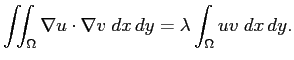
すなわち
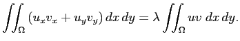
これを有限要素法で離散化すると、一般化固有値問題と呼ばれる
という形をした方程式が得られる。 ここで
「シフト法で解く」と簡単に書いてあるだけで、詳しいことは書いてない。
次のようなことかと推測する。
一般化固有値に近いと考えられる実数 ![]() を与えたとき、
を与えたとき、
![]() の両辺から
の両辺から
![]() を引くと、
を引くと、
ゆえに
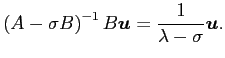
これは
 に属する固有ベクトルであることを示す。
ゆえに行列
に属する固有ベクトルであることを示す。
ゆえに行列
 が得られる。
細かいことだが、重要な注意がある。
ここでは square() を用いてメッシュ分割をしているが、
それを用いずに、自分で境界曲線を定義してメッシュ分割をすると、
真の固有値が重複(縮重)する場合であっても、
数値計算で得られる近似固有値は重複(縮重)しない。
これは自動メッシュ分割で得られる三角形分割は、
正方形の二面体群 (合同変換全体のなす群) ![]() の対称性を持たないため、
近似固有値が重複しないためである。
の対称性を持たないため、
近似固有値が重複しないためである。