Next: 10.5 LU分解, Cholesky分解 Up: 10 線形演算 Previous: 10.3.1 注意
標準ライブラリィに疎行列用の SparseArrays というものがある。 使い方は、Sparse Arrays を読むと良い (この解説はちゃんとしている)。
using SparseArrays |
sparse() で普通の Array を SparseArray に出来る。 SparseArray を普通の Array にするには Array() あるいは collect() を用いる。
julia> A = sparse([1 2 0; 0 0 3; 0 4 0])
3×3 SparseMatrixCSC{Int64,Int64} with 4 stored entries:
  [1, 1]  =  1
  [1, 2]  =  2
  [3, 2]  =  4
  [2, 3]  =  3

julia> Array(A)
3×3 Array{Int64,2}:
 1  2  0
 0  0  3
 0  4  0
|
“SparseMatrixCSC” の CSC は、“Compressed Sparse Column” の略である。
まず Compressed Column 形式を説明する。 行列
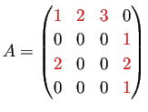
こう書く方が分かりやすいかな?
|
から
|
|
| Compressed Column 形式で行列を作る |
julia> IA=[1,3,1,1,2,3,4]; JA=[1,1,2,3,4,4,4]; VA=[1,2,2,3,1,2,1];
julia> a=sparse(IA,JA,VA)
4×4 SparseMatrixCSC{Int64,Int64} with 7 stored entries:
  [1, 1]  =  1
  [3, 1]  =  2
  [1, 2]  =  2
  [1, 3]  =  3
  [2, 4]  =  1
  [3, 4]  =  2
  [4, 4]  =  1

julia> A=collect(a)
4×4 Array{Int64,2}:
 1  2  3  0
 0  0  0  1
 2  0  0  2
 0  0  0  1
|
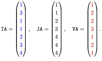
(ある意味で不要であるが、練習として) 次に Compressed Row 形式を説明する。
まず非零要素を上から下、左から右に検索し3、行番号、列番号、非零要素のベクトルを作る。
まず第1行の
![]() 列に
列に
![]() ,
続いて第2行の
,
続いて第2行の
![]() 列に
列に
![]() ,
第3行の
,
第3行の
![]() 列に
列に
![]() ,
第4行の
,
第4行の
![]() 列に
列に
![]() がある。
これから
がある。
これから
言い換えると
|
から
|
|
| Compressed Row 形式で行列を作る |
julia> IA=[1,1,1,2,3,3,4]; JA=[1,2,3,4,1,4,4]; VA=[1,2,3,1,2,2,1];
julia> a=sparse(IA,JA,VA)
4×4 SparseMatrixCSC{Int64,Int64} with 7 stored entries:
  [1, 1]  =  1
  [3, 1]  =  2
  [1, 2]  =  2
  [1, 3]  =  3
  [2, 4]  =  1
  [3, 4]  =  2
  [4, 4]  =  1

julia> A=collect(a)
4×4 Array{Int64,2}:
 1  2  3  0
 0  0  0  1
 2  0  0  2
 0  0  0  1
|
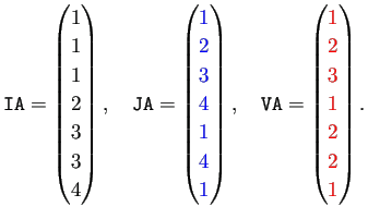
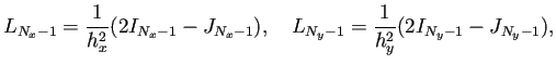
では、Compressed Sparse Column 形式の説明をする。
Compressed Row 形式では IA が、
Compressed Column 形式では JA が、重複の多いベクトルになりがちである。
例えばCompressed Column 形式で、上の例では JA=[1,1,2,3,4,4,4]で
あり、![]() と
と ![]() が重複している。
が重複している。
![]() が最初に現れるのは
が最初に現れるのは ![]() 番目、
番目、
![]() が最初に現れるのは
が最初に現れるのは ![]() 番目、
番目、
![]() が最初に現れるのは
が最初に現れるのは ![]() 番目、
番目、
![]() が最初に現れるのは
が最初に現れるのは ![]() 番目、この
番目、この ![]() だけを記憶しておけば、
JA は再生できる。
この方法を Compressed Sparse Column 形式 (CSC) と呼ぶ。
だけを記憶しておけば、
JA は再生できる。
この方法を Compressed Sparse Column 形式 (CSC) と呼ぶ。
Julia の Sparse Array では、 この Compressed Sparse Column 形式がデータ構造に採用されているそうだ。
以上、データ構造の話をしたけれど、次の応用例は、 データ構造を知らなくても理解できる (笑)。
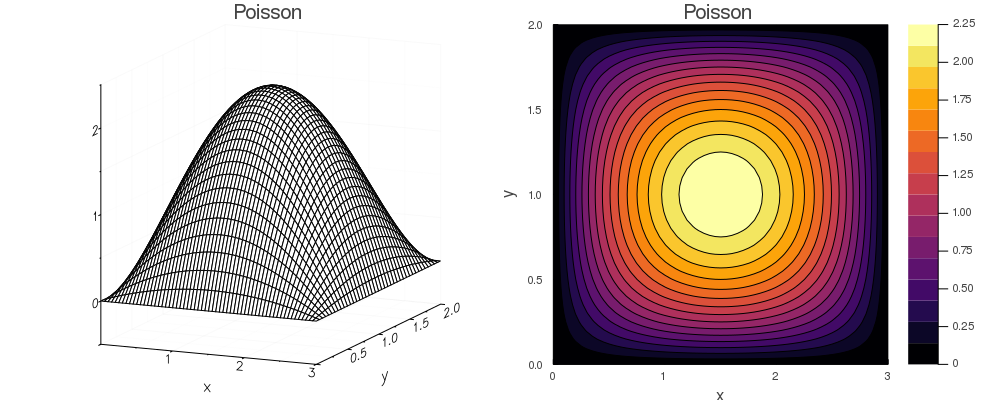
例題
長方形領域
![]() における Poisson 方程式を、
差分法で解いてみよう。
における Poisson 方程式を、
差分法で解いてみよう。
 | ||
 | ||
 |
(詳しいことは、例えば 「Poisson方程式に対する差分法」 を見よ。)
MATLABでは、次のようなプログラムを書いた。
| poisson_coef.m |
function A=poisson_coef(W, H, nx, ny) % 長方形領域 (0,W)×(0,H) における Poisson 方程式の Dirichlet 境界値問題 % Laplacian を差分近似した行列を求める。 % 長方形を nx×ny 個の格子に分割して差分近似する。 % MATLABでは % (1) 行列は Fotran と同様の column first であり、 % (2) mesh(), contour() による「行列描画」は Z(j,i) と添字の順が普通と逆なので、 % l=i+(j-1)*(nx-1) と row first となるように1次元的番号付けする hx=W/nx; hy=H/ny; m=nx-1; n=ny-1; ex=ones(nx,1); ey=ones(ny,1); Lx=spdiags([-ex,2*ex,-ex],-1:1,m,m)/(hx*hx); Ly=spdiags([-ey,2*ey,-ey],-1:1,n,n)/(hy*hy); A=kron(speye(m,m),Ly)+kron(Lx,speye(n,n)); |
| poisson_coef.m |
% 長方形領域 (0,W)×(0,H) で Poisson 方程式の同次Dirichlet境界値問題を解く
W=3.0;
H=2.0;
nx=30;
ny=20;
m=nx-1;
n=ny-1;
% 連立方程式を作成して解く
% MATLABの行列は Fotran と同様の column first であり、
%「行列描画」は Z(j,i) と添字の順が普通と逆なので、
% l=i+(j-1)*(nx-1) と row first となるように1次元的番号付けする
A=poisson_coef(W, H, nx, ny);
%
x=linspace(0,W,nx+1); % x=[x_0,x_1,...,x_nx]
y=linspace(0,H,ny+1); % y=[y_0,y_1,...,y_ny]
[X,Y]=meshgrid(x,y);
% f≡1 の場合
%F=ones(m*n,1);
f=-2*(X.^2-3*X+Y.^2-2*Y);
f=f(2:ny,2:nx);
F=f(:);
%
U=zeros(n,m);
U(:)=A\F;
% 境界値0をつける
u=zeros(ny+1,nx+1);
u(2:ny,2:nx)=U;
%
% グラフの鳥瞰図
clf
colormap hsv
subplot(1,2,1);
mesh(X,Y,u);
colorbar
% 等高線
subplot(1,2,2);
contour(X,Y,u);
%
disp('図を保存する');
print -dpdf poisson2d.pdf % 利用できるフォーマットは doc print で分かる
print -dpng poisson2d.png % 利用できるフォーマットは doc print で分かる
print -deps poisson2d.eps % 利用できるフォーマットは doc print で分かる
|
Julia で同じことをうまくやるにはどうすれば良いか、 イマイチ分からないが、とりあえず以下で実現できる。
# poisson2d.jl --- 長方形 Ω=(0,W)×(0,H) における -△u=f, u=0 (on ∂Ω)
#=
元はMATLABプログラム
http://nalab.mind.meiji.ac.jp/~mk/labo/text/new-intro-matlab/node8.html
using LinearAlgebra
using SparseArrays
using Plots
gr()
include("poisson2d.jl")
=#
# MATLABの真似…でも要らない?
# 参考 https://qiita.com/yshutaro/items/54d64c406f624545429a
# xx,yy=meshgrid(x,y); fv=f.(xx,yy) の代わりに fv=f.(x',y) でOKとか
function meshgrid(x,y)
m=size(x)[1]
n=size(y)[1]
ones(n)*x',y*ones(m)'
end
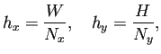
function poisson_coef(W, H, nx, ny)
hx=W/nx
hy=H/ny
m=nx-1
n=ny-1
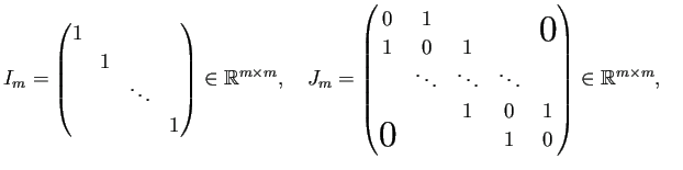
Lx=SymTridiagonal(2.0*ones(m),-ones(m-1))/(hx*hx)
Ly=SymTridiagonal(2.0*ones(n),-ones(n-1))/(hy*hy)
kron(sparse(1.0I,m,m),sparse(Ly))+kron(sparse(Lx),sparse(1.0I,n,n))
end
# Poisson方程式の右辺
function f(x,y)
-2*(x^2-3*x+y^2-2*y)
end
function poisson2d(W=3.0, H=2.0, nx=60, ny=40)
# W=3;H=2;nx=6;ny=4;
println("W=$W, H=$H, nx=$nx, ny=$ny")
m=nx-1
n=ny-1
A=poisson_coef(W, H, nx, ny)
x=range(0.0, W, length=nx+1)
y=range(0.0, H, length=ny+1)
if (false)
xx,yy=meshgrid(x,y) # xx, yy は (ny+1)×(nx+1) Array になる
fv=f.(xx,yy) # fv[j,i] は f の xi,yj での値
else
fv=f.(x',y) # fv[j,i] は f の xi,yj での値
end
F=reshape(fv[2:end-1,2:end-1],(nx-1)*(ny-1),1) # 内部格子点での値を1次元化
u=zeros(ny+1,nx+1)
u[2:end-1,2:end-1]=reshape(A\F,ny-1,nx-1)
#
p1=plot(x,y,u,st=:wireframe,
xaxis=("x"),yaxis=("y"),zaxis=("u",(-0.2,2.2)),title="Poisson")
#
p2=plot(x,y,u,st=:contour,fill=true,
xaxis=("x"),yaxis=("y"),zaxis=("u",(-0.2,2.2)),title="Poisson")
#
p=plot(p1,p2,layout=(1,2),size=(1000,400))
savefig("poisson2d.svg"); savefig("poisson2d.pdf"); savefig("poisson2d.png")
display(p)
end
|
| 試してみよう |
curl -O http://nalab.mind.meiji.ac.jp/~mk//misc/20200102/poisson2d.jl
julia
using Plots
using LinearAlgebra
using SparseArrays
include("poisson2d.jl")
poisson2d()
|
Julia には、MATLAB の speye() や eye() に相当する関数はない。 単位行列が必要ならば、operator I を使いなさい、とか。 そこで sparse(1.0I,n,n) を speye(n,n) の代わりに使っている。 Lx や Ly に sparse() を作用させるのが大事で、 最初
Lx=SymTridiagonal(2.0*ones(m),-ones(m-1))/(hx*hx) Ly=SymTridiagonal(2.0*ones(n),-ones(n-1))/(hy*hy) A=kron(sparse(1.0I,m,m),Ly)+kron(Lx,sparse(1.0I,n,n)) |
桂田 祐史