


Next: B. sample1.edp, sample2.edp, sample3.edp Up: 応用複素関数レポート課題2 Previous: 6 流線を描くために: 流れ関数 を求める
(これは場合分けの不要な単純なプログラムである。)
サンプルプログラム sample0.edpでは、
単位円盤領域
 における一様流
 の場合のプログラムである。
単位円盤なので
の場合のプログラムである。
単位円盤なので
 (ここは良く考えること。
例えば楕円の場合は
(ここは良く考えること。
例えば楕円の場合は  はかなり複雑な式になる。).
これから
はかなり複雑な式になる。).
これから
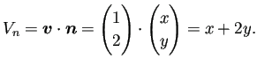
( が
が  で定数関数なので)
 であるから、
当然
であるから、
当然
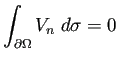 も成り立つ。
| sample0.edp |
// sample0.edp
//   https://m-katsurada.sakura.ne.jp/complex2/sample0.edp
//   2次元非圧縮ポテンシャル流
//     速度ポテンシャル,速度を求め、等ポテンシャル線, 速度場を描く

border Gamma(t=0,2*pi) { x = cos(t); y = sin(t); } // 円盤領域
int m=64;
mesh Th=buildmesh(Gamma(m));
plot(Th, wait=1, ps="Th.eps");
// 次の2行は区分1次多項式を使うという意味
fespace Vh(Th,P1);
Vh phi;
// 境界条件の設定
func Vn=x+2*y;// Ωが単位円で, V=(1,2) のとき V・n=x+2y
// 整合条件 ∫ V_n ds=0 のチェック
cout << "check the compatibility condition: " << int1d(Th,Gamma)(Vn) << endl;

// 有限要素法で連立1次方程式 A u=f を導く
varf Laplace(phi,v) =
  int2d(Th)(dx(phi)*dx(v)+dy(phi)*dy(v)) -int1d(Th,Gamma)(Vn*v);

matrix A = Laplace(Vh, Vh);
set(A,solver=CG);
real[int] f = Laplace(0, Vh); f = -f;
// fの定数成分(丸め誤差によるゴミ)を除く (Image A に射影する)
real[int] one(Vh.ndof);
one = 1.0;
one = one / sqrt(one' * one);
f=f-one'*f*one;
cout << "Does f belong to image space? (1, f)="<< (one' * f) << endl;

// 有限要素解を求める
phi[]=A^-1*f;

real meanphi=int2d(Th)(phi)/Th.area; // Th.area は int2d(Th)(1.0)
cout << "mean phi=" << meanphi << endl;
phi=phi-meanphi;
plot(phi,ps="contourpotential.eps",wait=1);

// ベクトル場 (v1,v2)=∇φ を描く (ちょっと雑なやり方)
Vh v1, v2;
v1=dx(phi); v2=dy(phi);
plot([v1,v2],ps="vectorfield.eps",wait=1);

// 等ポテンシャル線とベクトル場を同時に描く
plot([v1,v2],phi,ps="both.eps", wait=1);
|
![\includegraphics[width=10cm]{report2-prog/sample0.eps}](img61.png)