Next: 3.6 Python言語によるプログラム例 Up: 3 2次元の問題 Previous: 3.4 C++言語&Eigenによるプログラム例
Julia は 2012年に公開された新しいプログラミング言語で、 色々な特徴があるが、特に数値計算に向いているとされている。
Juliaの処理系のインストールの仕方は、付録 B を見よ。
参考のため1次元の問題のJuliaによるプログラムを掲げる。
| rk1ex1.jl |
# rk1ex1.jl --- dx/dt=x (0<t<1), x(0)=1 を Runge-Kutta法で解く

using Printf

function testrungekutta(Tmax=1.0,N=10)
  # 初期値
  t0=0.0
  x0=1.0
  #
  @printf("#N=%d Tmax=%f\n", N, Tmax)
  @printf("# t x\n")
  # Runge-Kutta法
  dt=Tmax/N
  t=t0
  x=x0
  for j=1:N
    k1=dt*f(t,x)
    k2=dt*f(t+dt/2, x+k1/2)
    k3=dt*f(t+dt/2, x+k2/2)
    k4=dt*f(t+dt, x+k3)
    x += (k1+2*k2+2*k3+k4) / 6
    t = j * dt
    @printf("%.4f %.7f\n", t, x)
  end
end

function f(t,x)
  x
end

# julia rk1ex1.jl と実行した場合に testrungekutta() を実行する。
if abspath(PROGRAM_FILE) == @__FILE__
    testrungekutta()
end
|
| 実行の仕方1 |
% julia rk1ex1.jl
#N=10 Tmax=1.000000 # t x 0.1000 1.1051708 0.2000 1.2214026 0.3000 1.3498585 0.4000 1.4918242 0.5000 1.6487206 0.6000 1.8221180 0.7000 2.0137516 0.8000 2.2255396 0.9000 2.4596014 1.0000 2.7182797 % |
| 実行の仕方2 |
% juliajulia> include("rk1ex1.jl") julia> testrungekutta(1,100) #N=10 Tmax=1.000000 # t x 0.1000 1.1051708 0.2000 1.2214026 0.3000 1.3498585 (中略) 0.9800 2.6644562 0.9900 2.6912345 1.0000 2.7182818 julia> |
次は van der Pol 方程式の問題のJuliaによるプログラムである。 Tmax, N を実行時に入力できるような工夫を入れてみた。
| rk2ex1.jl |
# rk2ex1.jl (Runge-Kutta method for van der Pol equation)
#
# 使い方
#   julia rk2ex1.jl              デフォルト Tmax=50, N=1000
#   julia rk2ex1.jl 100 2000     Tmax=100, N=2000
#   echo 'plot "rk2ex1.data" using 2:3 with l"' | gnuplot

using Printf

mu=1.0

# Runge-Kutta 法の1ステップ
function rungekutta(f,t,x,dt)
  k1=dt*f(t,x)
  k2=dt*f(t+dt/2, x+k1/2)
  k3=dt*f(t+dt/2, x+k2/2)
  k4=dt*f(t+dt, x+k3)
  x + (k1 + 2 * k2 + 2 * k3 + k4) / 6
end

# van der Pol 方程式の右辺
function f(t,x)
  y=similar(x)
  y[1]=x[2]
  y[2]=-x[1]+mu*(1.0-x[1]*x[1])*x[2]
  y
end

function testrungekutta(Tmax=50.0,N=1000)
  # 初期値
  t0=0.0
  x0=[0.1,0.1]
  #
  of=open("rk2ex1.data","w")
  # Runge-Kutta法
  dt=Tmax/N
  t=t0
  x=x0
  for i=1:N
    x=rungekutta(f,t,x,dt)
    t=i*dt
    s=@sprintf "%f %f %f\n" t x[1] x[2]
    print(s)
    print(of,s)
  end
  close(of)
end

# main
argc=length(ARGS)
if argc==0
        testrungekutta()
elseif argc==1
        testrungekutta(parse(Float64,ARGS[1]))
elseif argc==2
        testrungekutta(parse(Float64,ARGS[1]), parse(Int,ARGS[2]))
end
|
| 実行の仕方 |
|
% julia rk2ex1.jl
% gnuplot gnuplot> plot "rk2ex1.data" using 2:3 with l gnuplot> quit
% julia rk2ex1.jl 100 2000
|
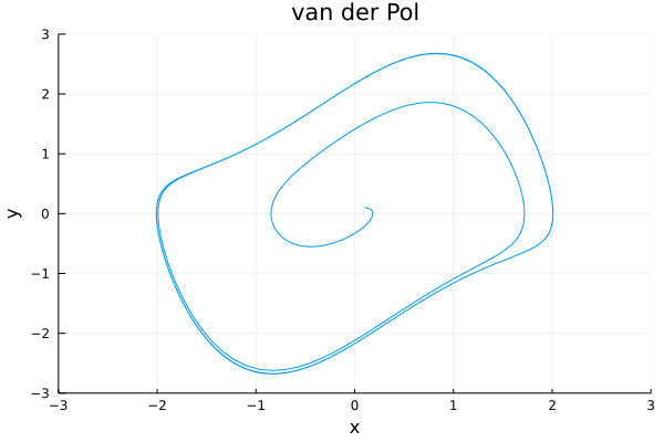
Julia には、グラフィックスのためのパッケージが色々ある。 Plots というパッケージを利用してグラフを描く機能を追加したのが、 次のプログラムである。
| rk2ex1plot.jl |
# rk2ex1plot.jl (Runge-Kutta method for van der Pol equation)
#
# 使い方
#   julia> include("rk2ex1plot.jl")
#   julia> testrungekutta()
#   julia> testrungekutta(10)
#   julia> testrungekutta(100,10000)

using Printf
using Plots

gr() # デフォルトがGRなので不要という説もある
mu=1.0

# Runge-Kutta 法の1ステップ
function rungekutta(f,t,x,dt)
  k1=dt*f(t,x)
  k2=dt*f(t+dt/2, x+k1/2)
  k3=dt*f(t+dt/2, x+k2/2)
  k4=dt*f(t+dt, x+k3)
  x + (k1 + 2 * k2 + 2 * k3 + k4) / 6
end

function f(t,x)
  y=similar(x)
  y[1]=x[2]
  y[2]=-x[1]+mu*(1.0-x[1]*x[1])*x[2]
  y
end

function testrungekutta(Tmax=50.0,N=1000)
  tv=zeros(N+1,1)
  xv=zeros(N+1,1)
  yv=zeros(N+1,1)
  # 初期値
  t0=0.0
  x0=[0.1,0.1]
  #
  of=open("rk2ex1.data","w")
  s="# Lotka-Volterrra equation"; println(s); println(of,s)
  s="# t x y"; println(s); println(of, s)
  # Runge-Kutta法
  dt=Tmax/N
  t=t0
  x=x0
  s=@sprintf "%f %f %f\n" t x[1] x[2]
  print(s)
  print(of,s)
  # 記録
  tv[1]=t; xv[1]=x[1]; yv[1]=x[2]
  # 時間を進める
  for i=1:N
    x=rungekutta(f,t,x,dt)
    t=i*dt
    tv[i+1]=t; xv[i+1]=x[1]; yv[i+1]=x[2]
    s=@sprintf "%f %f %f\n" t x[1] x[2]
    print(s)
    print(of,s)
  end
  close(of)
  p=plot(xv,yv,title="van der Pol",
         xaxis=("x"),yaxis=("y"),xlims=(-3,3),ylims=(-3,3),legend=false)
  savefig(p,"rk2ex1plot.png")
  display(p)
end

# main
println("usage:	testrungekutta()")
println("usage:	testrungekutta(10.0)          Tmax=10.0")
println("usage:	testrungekutta(500.0, 5000)   Tmax=500.0, N=5000")
|